Home Blogs & News

Interactively visualising DICOM volumes and header data

Digital Imaging and Communications in Medicine (DICOM) is an internationally recognised standard for medical imaging and is implemented in the majority of medical imaging devices today. DICOM standard is used across multiple imaging modalities, such as radiography, CT, MRI. Despite containing pixel information, DICOM files contain a lot of metadata about the image orientation, methods used to acquire an image, study and patient information, and more. This makes DICOM a valuable source in the field of medical visualisation, image analysis and research, as it allows its users to:

• visualise data and reconstruct 3D volumes
• perform image analysis workflows that might help to advance medical research
• easily combine imaging data with non-imaging data

In this post, I will discuss using oro.dicom and oro.nifty, packages which can be used to read DICOM files, interactively display volumes, and extract DICOM metadata. I will also create a mini-app with slider widgets which will allow me to change the position of the displayed slices. To do this I’ll be using an open BRAINIX dataset which contains DICOM images of a brain tumour and is available to download from Osirix DICOM image gallery.

Reading DICOM files

First off, let’s install the oro.dicom and oro.nifti packages and create the basis for our mini-app – the ui.r and server.r files.

ui.r

xap.require('oro.dicom','oro.nifti')

# Define UI space for our application
shinyUI(fluidPage(
  
  # UI code goes here
))

server.r

# Define server logic
shinyServer(function(input, output, session) {
  
   # Server code goes here
})

Now let’s prepare our data. Firstly I’ll unzip brainix.zip, and in this example, upload extracted DICOM files to the datafiles folder in my AnalytiXagility workspace via SFTP. Next I’ll define paths to individual DICOM image sets and use those as inputs in the selectInput() widget. This will allow me to interactively select which DICOM volume to display.

ui.r

fluidRow(
  column(width = 2,
    h5('Select DICOM file'),
    uiOutput('fileSelection')
  )
)

server.r

# Define server logic
shinyServer(function(input, output) {
  
  # Select path to DICOM files
  pth <- "~/datafiles/uploads/brainix/"
  # List folders the path (each folder contains a set of DICOM images)
  dirs <- list.dirs(path = pth, full.names = FALSE, recursive = TRUE)
  
  # Create drop-down menu to select DICOM sets
  output$fileSelection <- renderUI({
    selectInput('fileInput', '', choices = dirs, selected = dirs[2])
  })

})

Now I will add a reactive function to read a set of DICOM images into a reactive variable dcmImages using readDICOM() function, which reads multiple DICOM files which are located in a single directory, and creates an object containing DICOM header information, hdr and an array of image slices, img.

server.r

# Read set of DICOM images
  
dcmImages <- eventReactive(input$fileInput, {
  DICOM_source <-  paste(pth, input$fileInput, sep="")
  readDICOM(DICOM_source, verbose = TRUE)
})

Now, if we observe reactive dcmImages() and check the length of $hdr and $img we will see that length of both should be the same. Each element in the hdr list contains a dataframe with DICOM header information corresponding to each matrix or pixel array found in the img list, e.g. if we read “~/datafiles/uploads/brainix/SOUS – 702” set of DICOM images, we get 22 header entries for 22 image slices.

server.r

observe({
  # Get length of dcmImages() variables
  print(unlist(lapply(dcmImages(), length)))
})

## hdr img 
##  22  22

Visualising DICOM volumes

Now, since we can read sets of DICOM images, we want to display them in our mini-app. To do this I’ll use the dicom2nifty() function to convert the DICOM object to the NIFTI format – another popular format which incorporates affine coordinate definitions and creates a 3D volume from image slices based on what’s contained in the header. It is useful to work with Nifti as it makes it easier to display different viewing panes such as Axial, Sagittal and Coronal orientations.

I will add slider inputs for X, Y and Z coordinate with arbitrary min/max values. I’ll also create a tabset menu for Axial, Sagittal and Coronal viewing panes and define a plotOuptut in the new column.

ui.r

fluidRow(
  # Continue column UI element
  column(width = 2,
    h5('Select DICOM file'),
    uiOutput('fileSelection')
    #Add slider inputs with arbitrary min/max values 
    sliderInput('slider_x', 'X orientation', min=1, max=10, value=5),
    sliderInput('slider_y', 'Y orientation', min=1, max=10, value=5),
    sliderInput('slider_z', 'Z orientation', min=1, max=10, value=5)
  ),
      
# Adding column with plot display outputs
  column(width = 7,
    h5('Plane View'),
      tabsetPanel(type = "tabs", 
        tabPanel("Axial", plotOutput("Axial", height = "450px",   brush = "plot_brush")), 
        tabPanel("Sagittal", plotOutput("Sagittal", height = "450px",   brush = "plot_brush")), 
        tabPanel("Coronal", plotOutput("Coronal", height = "450px",   brush = "plot_brush"))
      )
    )
  )
)

In the server.r file, I’ll now create an observe function to update min/max values for slider inputs using updateSliderInput(), based on the dimensions [x,y,z] of the selected volume. I then pass positions of X, Y and Z slider inputs into the plot function and visualise the selected volumes in Axial, Sagittal and Coronal orientations. Using the oro.nifti subclass image we can just pass (“axial”, “sagittal”, “coronal”) value to plane parameter.

server.r

observe({
  volume <- niftiVolume()
  d <- dim(volume)

  # Control the value, min, max, and step.
  # Step size is 2 when input value is even; 1 when value is odd.
  updateSliderInput(session, "slider_x", value = as.integer(d[1]/2),max = d[1])
  updateSliderInput(session, "slider_y", value = as.integer(d[2]/2),max = d[2])
  updateSliderInput(session, "slider_z", value = as.integer(d[3]/2),max = d[3])
})
  
# Add Axial, Sagittal and Coronal displays
output$Axial <- renderPlot({
  try(image(niftiVolume(),  z = input$slider_z, plane="axial", plot.type = "single", col = gray(0:64/64)))
})
output$Sagittal <- renderPlot({
  try(image(niftiVolume(),  z = input$slider_x, plane="sagittal", plot.type = "single", col = gray(0:64/64)))
})  
  
output$Coronal <- renderPlot({
  try(image(niftiVolume(),  z = input$slider_y, plane="coronal", plot.type = "single", col = gray(0:64/64)))
})

The results at this point should look like this.

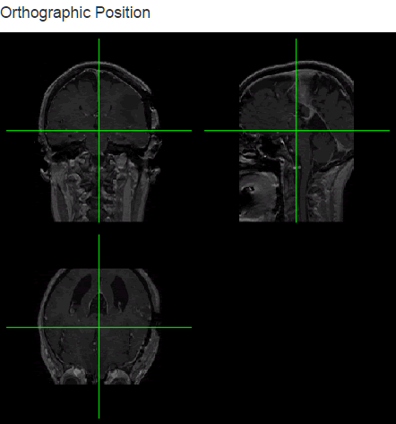
We can also include orthographic view using the orthographic() function and pass our slider positions as arguments for X, Y and Z positions. I will create a plot output object using plotOutput("orthographic", "Orthographic view") and add a reactive plot to create an orthographic view with crosshairs.

server.r

output$orthographic<- renderPlot({
  orthographic(niftiVolume(),
               col.crosshairs="green",
               xyz = c(input$slider_x,   input$slider_y, input$slider_z),
               oma = rep(0, 4),
               mar = rep(0.5, 4),
               col = gray(0:64/64)
  )
})

Working with DICOM header

Finally, I’m going to extract useful information contained in the DICOM header. I will create a list of header elements I want to extract, containing the “StudyID”, “StudyDescription”, “ProtocolName”, “Modality”, “PatientsName”, “PatientID” tags. You can find the extensive list of DICOM header tags here. I then apply the extractHeader() function to my list and pass the dcmImage object as a parameter. Then I select the row which corresponds to the currently displayed image.

server.r

output$header <- renderTable({
  validate(
    need(length(dcmImages()) >1,  "Please select a data set")
  )
    
  tags <- c("StudyID", "StudyDescription", "ProtocolName", "Modality", "PatientsName", "PatientID")
  SliceHeader <- data.frame(sapply(tags, extractHeader, hdrs=dcmImages()$hdr, numeric=FALSE))[input$slider_z,]
})

Personally I prefer to view DICOM images on darker backgrounds – if you would like to do the same you can define a CSS file or download a free bootswatch theme. Here, I’m using the Superhero theme as theme.css, placing it in the www folder of my mini-app. By simply adding theme = "theme.css" in the ui.r I get a darker look to my DICOM viewing application.

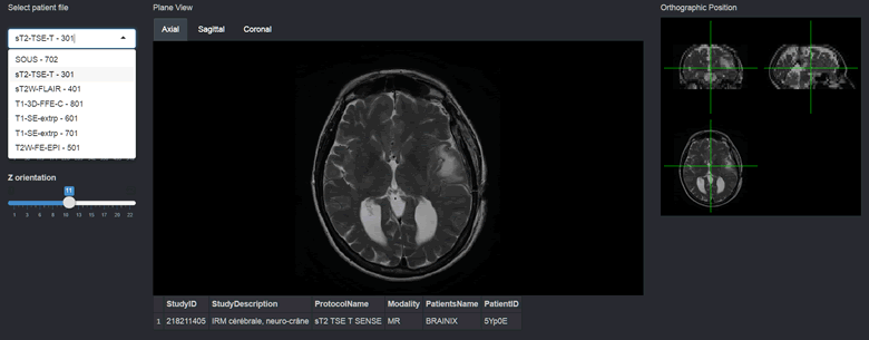
In this post, I presented a way to interactively visualise slices and header information from sets of DICOM images using oro.dicom and oro.nifti packages. In the future, I will be looking into adding JavaScript-based keyboard and mouse controls, as well as some image analysis elements.

Let me know if there’s anything you would like to see me cover in future posts – I like a challenge!