Home Blogs & News

Analysing larger-than-memory datasets efficiently in R

Aridhia DRE workspaces come with everything you need out of the box to do very large scale data analysis without the need to use a virtual machine. Pre-loaded packages support working with scalable file types and deploying packages efficiently.

In this blog, Kim Carter, Chief Data Officer at Aridhia, gives us some examples of how to do this and make your analysis more efficient and scalable. With examples of:

• Big-data at laptop scale: >200 million rows processed in R in our DRE environment or on your laptop without the need for big VM or HPC, requires 2-3GB of RAM only
• Massive storage gain: 78 GB of raw data → 10 GB using Parquet, enabling high-speed random access and columnar reads.
• Full compatibility: Works seamlessly with tidyverse-style pipelines via arrow::open_dataset().
• Zero-copy analytics: Queries operate directly on Parquet files without full in-memory loading.

Background on dataset

This analysis uses the NHS England Prescribing Data, which provides monthly records of all NHS primary-care prescriptions dispensed in England. Each monthly file represents every GP practice across the country, with detailed cost, volume, and classification data for each prescribed drug.

• Coverage: 12 consecutive monthly datasets, from June 2024 to May 2025
• Raw format: 12 × CSV (~6.5 GB each) → ~78 GB total uncompressed
• Converted format: Apache Parquet (~600–700 MB each) → ~10 GB total
  → ≈ 8× compression while retaining full precision and columnar structure
• Number of records: ~17 million per month (~200 million+ overall)
• Fields include:
  • YEAR_MONTH — reporting period (YYYYMM)
  • REGIONAL_OFFICE_NAME, ICB_NAME, PRACTICE_NAME, POSTCODE — geography & practice identifiers
  • BNF_CODE, CHEMICAL_SUBSTANCE_BNF_DESCR, BNF_DESCRIPTION — prescribing classification
  • QUANTITY, ITEMS, ACTUAL_COST, NIC — volume and cost metrics

Tip: when downloading the NHS monthly files in .zip format, if the NHS zips won’t unzip for you, trying p7zip (the files a newer zip version).

Data source: NHS England Open Data Portal – Prescribing Data. Note this dataset has just been updated to now include new standardised SNOMED codes, read more on the link.
Contains public sector information licensed under the Open Government Licence v3.0.

Prerequisites

Make sure you have the following R packages installed:

• arrow (with dataset support)
• dplyr /li>
• ggplot2
• A recent version of R (4.2+ recommended)

Aridhia’s DRE workspaces already have all of these packages pre-installed, so you can quickly get code running.

Installing R Packages Quickly Using RSPM

When working with R in a secured or resource-limited environment, package installation time can easily become a bottleneck, especially for larger packages that require compilation from source. To make this faster and more reliable, you can use RSPM as the primary package source.

RSPM provides pre-built Linux binaries for a large subset of CRAN and Bioconductor packages, falling back to source builds only when binaries are not available. This means:

• Package installation is dramatically faster
• No need for compilers or build toolchains for most packages
• Less time spent resolving system dependencies
• Greater consistency across users and workspaces

In our DRE, RSPM is installed by default; otherwise you can simply run:

install.packages(“rspm”)

If a pre-built package for your platform exists, RSPM will automatically download it; if not, it will build from source as usual.

rspm:enable() 
install.packages(“ggplot2”) 

If a pre-built package for your platform exists, RSPM will automatically download it; if not, it will build from source as usual.

Converting CSVs to Parquet files

Before doing any analysis, the first and most important step is converting the raw NHS CSV files into Apache Parquet. The CSVs are huge (around 6.5 GB each, ~78 GB for 12 months) and cannot be handled memory efficiently in R using traditional methods like read.csv or read_csv, which read straight to RAM and will quickly crash out on most machines.

Parquet is a compressed, column-oriented format that reduces the dataset CSVs to around 600–700 MB per month (~10 GB total) while enabling fast, low-memory access through Arrow.

It takes just under a minute for each file to be converted and compressed into ~600MB parquet file (on a average machine), as a one-off activity.

The code below gets a list of .csv files (you can amend to specify a full path to the downloaded files), and for each file converts file through to parquet format using arrow:

library(arrow) 
csv_files <- list.files(pattern = "\\.csv$") 
for (csv in csv_files) 
{ 
    parquet_file <- sub("\\.csv$", ".parquet", csv) 
    ds <- open_dataset(csv, format = "csv") 
    write_dataset(ds, path = parquet_file, format = "parquet") 
    rm(ds); gc() # Clean up after each file 

Tip: use a clean, empty output directory.

Arrow’s open_dataset() will later treat every file under that directory as part of the Parquet dataset.
If stray CSVs are left in there, the dataset will fail to load.

High-Performance Analysis on the Full 200M+ Row Dataset

With all twelve monthly CSV files converted to Parquet, we can now load the entire year of NHS prescribing data as a single Arrow dataset (ds) and begin analysing it directly on disk. Because Arrow evaluates operations lazily and reads only the columns required, we can work efficiently across more than 200 million rows using ordinary R code and familiar dplyr syntax without ever loading the full dataset into memory.

The four tasks are:

1. Quick data summary: a fast, high-level overview of the dataset (record counts, monthly totals).
2. Top regions: identifying the NHS regional offices with the highest prescribing activity.
3. Top drugs: ranking the most costly chemical substances across the entire year.
4. Monthly prescribing trends for Semaglutide: extracting and visualising month-by-month trends for one of the most clinically and commercially relevant medicines for managing type-2 diabetes.

Task 1: Dataset summary

# load the parquet files if not already loaded 
# ds <- open_dataset("/home/workspace/files/NHSDATA/", format = "parquet") 

# calculate total number of rows and columns 
# without loading all of the data (takes a few seconds) 
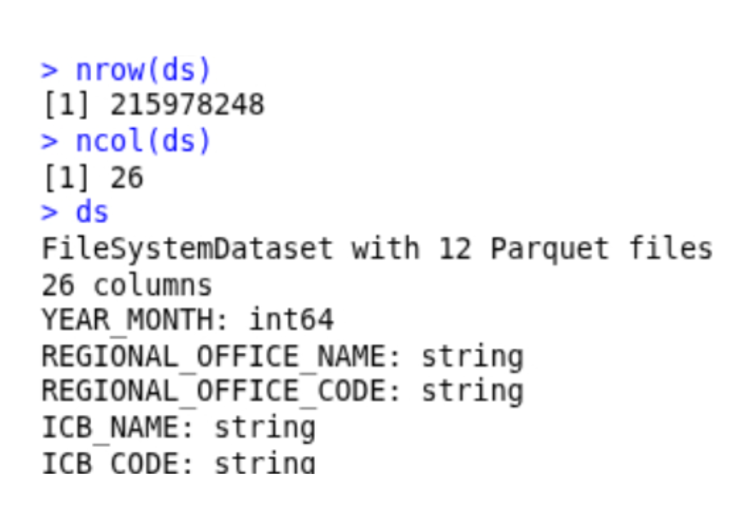
nrow(ds) 
ncol(ds) 
ds # summary of the ds object 
 
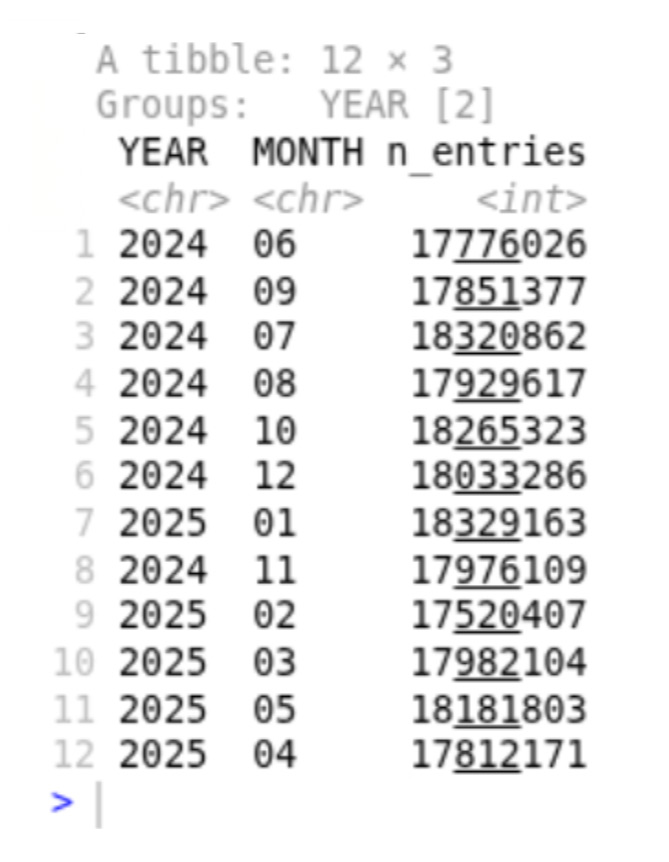
# summarise data by year and month 
ds %>% 
  mutate( 
    YM_STR = cast(YEAR_MONTH, string()), 
    YEAR = substr(YM_STR, 1, 4), 
    MONTH = substr(YM_STR, 5, 6) 
  ) %>% 
  group_by(YEAR, MONTH) %>% 
  summarise(n_entries = n()) %>% 
  collect()

Which returns a brief overview of our 215M row x 26 column dataset, with the number of prescriptions per year and month summarised. It takes about 20-30 seconds on an average computer.

Task 2: Top prescribing regions

# summarise the total prescriptions by regions, then sort 
top_regions <- ds %>% 
  group_by(REGIONAL_OFFICE_NAME) %>% 
  summarise(total_items = sum(ITEMS, na.rm = TRUE)) %>% 
  arrange(desc(total_items)) %>% 
  head(12) %>% 
  collect()  

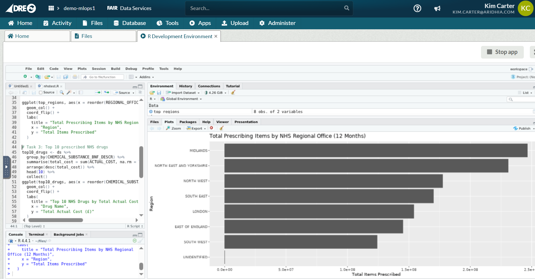
ggplot(top_regions, aes(x = reorder(REGIONAL_OFFICE_NAME, total_items), y = total_items)) + 
  geom_col() + 
  coord_flip() + 
  labs( 
    title = "Total Prescribing Items by NHS Regional Office (12 Months)", 
    x = "Region", 
    y = "Total Items Prescribed" 
  ) 

As with Task 1, it takes 20-30 seconds to summarise the dataset by regions, with Midlands and the North & East Yorkshire regions leading the way in prescription counts (June 24-May25) despite Greater London having a significantly larger population.

Task 3: Top prescribed drugs by total Cost

# summarise top drugs by descending cost 
top10_drugs <- ds %>% 
  group_by(CHEMICAL_SUBSTANCE_BNF_DESCR) %>% 
  summarise(total_cost = sum(ACTUAL_COST, na.rm = TRUE)) %>% 
  arrange(desc(total_cost)) %>% 
  head(10) %>% 
  collect() 

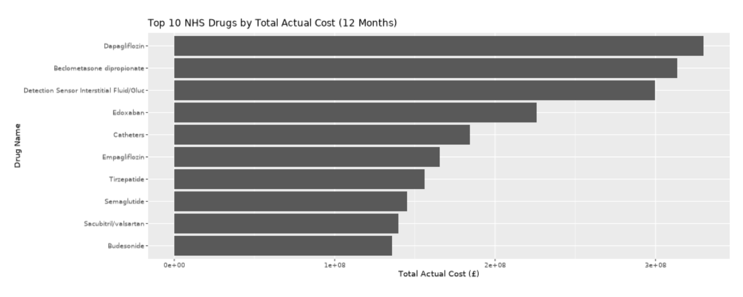
ggplot(top10_drugs, aes(x = reorder(CHEMICAL_SUBSTANCE_BNF_DESCR, total_cost), y = total_cost)) + 
  geom_col() + 
  coord_flip() + 
  labs( 
    title = "Top 10 NHS Drugs by Total Actual Cost (12 Months)", 
    x = "Drug Name", 
    y = "Total Actual Cost (£)" 
  )

Next, we’ll tally up the top prescribed drugs by total cost, such that the most prescribed drugs are not necessarily those with the highest cost burden. This type of calculation again requires processing all of the rows of data in multiple ways, and can be done efficiently via arrow & the parquet files we’re created. Number one is Dapagliflozin (under trade names like Farxiga and Forxiga), coming in at £330M GBP for the period Jun 24-May 25. The drug helps your kidneys remove sugar from your blood, and is used in the management of type 2 diabetes and patients with heart failure or chronic kidney disease.

Task 4: Prescriptions for Semaglutide (Ozempic)

# Prescription counts for Ozempic 
drug_of_interest <- "Semaglutide" 

monthly_drug <- ds %>% 
  filter(CHEMICAL_SUBSTANCE_BNF_DESCR == drug_of_interest) %>% 
  mutate( 
    YM_STR = cast(YEAR_MONTH, string()), 
    YEAR = substr(YM_STR, 1, 4), 
    MONTH = substr(YM_STR, 5, 6), 
    YEAR_MONTH_LABEL = paste0(YEAR, "-", MONTH) 
  ) %>% 
  group_by(YEAR_MONTH_LABEL) %>% 
  summarise(total_items = sum(ITEMS, na.rm = TRUE)) %>% 
  arrange(YEAR_MONTH_LABEL) %>%
 collect() 

ggplot(monthly_drug, aes(x = YEAR_MONTH_LABEL, y = total_items, group = 1)) + 
  geom_line() + 
  geom_point() + 
  labs(
    title = paste0("Monthly Prescribing Trend: ", drug_of_interest), 
    x = "Year-Month", 
    y = "Total Items Prescribed" 
  ) + 
  theme(axis.text.x = element_text(angle = 90, hjust = 1))

Finally, we’ll dive into the prescription patterns for a single drug, Semaglutide otherwise known as Ozempic/Wegovy and so on by tradename (number 8 on the list above). Without diving into any formal statistical tests, there’s a rough decline over the 12 month period, which may reflect global shortages in supply and changing regulations by the General Pharmaceutical Council.

Within our DRE R environment, or similar on a laptop with < 10GB of RAM, I’ve analysed more than 200 million NHS records seamlessly and efficiently in R using Parquet and Arrow. Peak memory usage during even the largest group-by queries never exceeded 2.5GB. This is big data analytics, made accessible to all.