Blogs & News
Beauty in Simplicity – Visualising Large-scale Genomic Data
If you’ve spent any time looking into the visualisation of large-scale genomic data then you’ve probably encountered Circos, a visualisation tool developed for displaying and analysing the large data output of genome sequencing. If not, you may still have unwittingly come across some of the many visualisations out there using Circos, or employing the same central ideas, to show anything from worldwide migration to mathematical art to (ostensibly) dinosaur genomes. These types of plots show a blend of functionality and form where your data visualisations can become striking showpieces while simultaneously delivering insights into your data.
In this post I’m going to show you how we can add a layer of interactivity to a Circos style plot from within AnalytiXagility using the excellent R packages, Shiny by RStudio and ggvis that we’ve integrated into the platform, and open data downloaded from the International Cancer Genome Consortium.
ICGC genome browser
The data used in the mini-app we developed in AnalytiXagility to prototype some of the ideas described is this post is from the International Cancer Genome Consortium (ICGC), specifically data from the Pancreatic Cancer – Ductal Adenocarcinoma (PACA-AU) project led by Sean M. Grimmond and Andrew V. Biankin.
Several datasets are made available for download which are the downstream results of various genomic analysis techniques. The data we used for our mini-app are the results of somatic variant analysis and include single nucleotide polymorphisms, structural variation and copy number variation.
Single nucleotide polymorphisms are where a single base within the genome has been altered relative to some standard, while structural and copy number variations (really just a form of structural variation) are instances in which larger sections of DNA have been moved, inverted, duplicated or lost, again relative to some standard. In the case of somatic analysis, the DNA we are looking at is from tumour tissue of the donor and the standard we are comparing against is the DNA from their healthy tissue.
In order to create the mini-app, we first uploaded the data to AnalytiXagility and filtered it to contain only the donor data for which the datasets described above were available. Next, we built up a general framework for creating circular visualisations using ggvis, while keeping in mind that we would want this to interact nicely with Shiny to introduce an extra layer of interactivity on top of what ggvis already offers. Finally, we integrated this work with the mini-apps capability within AnalytiXagility using Shiny to create an interactive Circos-style visualisation of each donor’s genome.
Play the video below to get a quick overview of the mini-app or try it out for yourself on the Shiny showcase.
Why circular visualisations?
There are advantages to using a circular visualisation in certain circumstances. I’ll outline a few of these here, along with a few disadvantages or areas where interactivity can improve on the interpretability of the plot. Generally a Circos plot is composed of several tracks, each of which can contain a different plot. Each track can also be split into several segments relative to the size of the object they are representing so that each segment of the circle contains data from a single object. The interior of the plot is then usually used to link together to show relationships between the objects or specific positions within the objects.
Pros
- Effective at showing interactions between objects or positions; Circos plots give an obvious way to organise links between objects without having them intersect other objects in the plot.
- Easy to show many different plots with the same x-axis scale (e.g. genomic position) in the same image.
- Increases the length of your x-axis allowing you to show things with greater fidelity than would be possible on a normal plot in Cartesian coordinates. Combining this with the previous point, objects towards the outside of the plot can be shown in higher resolution than those towards the inside, so there is an effective way to provide both summary statistics and precise positions on the same plot.
- For data with an inherent circular aspect to them (e.g. time of day, time of year, microbial genomes), distances between points are preserved in the plot.
- The plots are engaging and encourage further investigation.
Cons
- Radial coordinates can be confusing; up and down become relative to where you are on the circle, so it can be difficult to compare quantities in different parts of the plot. Appropriate radial grids can make this easier, but it’s still not as natural as in cartesian coordinates.
- Decreases the length of your y-axis; if you have several tracks with different plots then each of these will only have a fraction of the radius of the circle to use as a y-axis. Generally, it is best to stick to plots without a y-axis, or plots where the fine detail in the y-axis isn’t that important.
- It’s easy to get carried away with creating a visually striking plot which ultimately conveys very little information or detracts from what the plot is trying to show. Of course, this is true of any visualisation, but it applies more here than for other, more standard, plots.
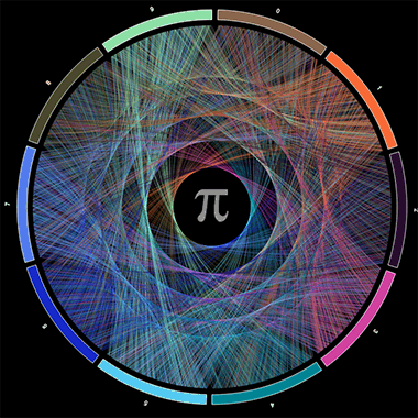
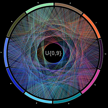
The last points in each list are really just the same point with different inflections and whether it’s a pro or a con depends on how you present your visualisation. As an example (and an opportunity to pay homage to Cristian Ilies Vasile’s and Martin Krzywinski’s beautiful visualizations involving mathematical constants), I’m going to recreate some mathematical art visualising pi and compare it to an (almost certainly) alternate sequence of numbers using R and ggvis.
These plots are certainly beautiful and engaging and make you want to dive in further and this comparison may even elicit further questions. However, if these plots were presented in a context where being able to quickly tell the difference between each or being able to extract precise details from each link was important, then they obviously fall flat. In fact, if the labels in the centre were removed you’d be hard pressed to tell which was which, while the raw data (the actual sequence of numbers) would answer this question almost immediately.
Introducing interactivity
The Shiny by RStudio package that we recently integrated into AnalytiXagility allows you to quickly build up interactive apps (see our other app development posts for more detail). Adding ggvis into the mix allows even more interactivity in the form of tooltips; events that occur when you click or hover over part of the plot and smooth, and even aesthetically pleasing, transitions between different plot states. You can quickly and easily build up a working prototype app directly from R, and this provides a particularly natural progression if initial analysis has already been performed in R.
I’m going to give a few examples of the interactivity we can add to a Circos style plot in a genomic context within AnalytiXagility.
Changing the data
Probably the simplest example aspect of interactivity and not really specific to circular plots. We keep the same framework and plot different data on it. In a genomic context you could have several different samples that have each gone through the same analysis where you want to be able to switch between the results of each.
Resizing and splitting
Even though circular plots increase the length of your x-axis, when trying to visualise something as large as the entire human genome, single pixels on your screen will end up containing several kB of the genome. We can partially solve this problem by allowing dynamic zooming or resizing of certain elements in the plot, although objects on the scale of the human genome would require a lot of zooming to get to even a one position per pixel scale.
Similarly, we can also expand the y-axis of certain tracks or split regions into smaller constituent parts.
Tooltips
We can entirely circumvent the issue with resolution described above by adding tooltips to the visualisation so that the plot itself gives a general overview of where and what things are, and clicking or hovering over them will tell you exactly where and what they are.
Additionally, objects in genomic visualisations – such as genes or single point mutations – can have a huge amount of information behind them that wouldn’t be possible to show in the plot. There are vast online databases, such as Clinvar or Ensembl, containing information on these objects that we can link to through tooltips, allowing further exploration from the visualisation.
Making the plot part of your UI
An application can contain more than one plot and we can link plots together in an AnalytiXagility mini-app so that one controls what is shown on the other. Using this idea we can turn a Circos visualisation into part of the user interface where we can use it to identify areas of interest, and then select those areas to look at in further detail using different plots.
What’s next
There’s so much more to say on this subject, so I’m going to follow up with another post next week, where I’ll be describing some of the technical details on how ggvis and Shiny can be used to create these Circos-style visualisations within AnalytiXagility. In the meantime please feel free to leave a comment below if you have any questions, and remember that you can try the visualisation out for yourself at the Shiny showcase.
Circos: An information aesthetic for comparative genomics
Martin I Krzywinski, Jacqueline E Schein, Inanc Birol, Joseph Connors, Randy Gascoyne, Doug Horsman, Steven J Jones, and Marco A Marra
Genome Res. Published in Advance June 18, 2009, doi:10.1101/gr.092759.109